This notebook seeks to help you set up your environments, get coiled set up, and learn the insides of key functions, and then use my libraries built on top of CalAdapt’s climatekitae!
ToC
| Part | What | Time |
|---|---|---|
| 0 | Docker | ~8 min first time, 0.5 mins thereafter |
| 1 | Coiled setup | ~7 min |
| 2 | Fetch climate data with the library | 5 min |
| 3 | Understand key functions | 4 min |
| 4 | Exercise — fetch data for a new park | 10 min |
| 4.5 | Saving to CSV-- plotting in R, final summary | 5 min |
Start (container)
Prerequisites: Docker Desktop installed + the VS Code Dev Containers extension (ms-vscode-remote.remote-containers).
Option A — VS Code (recommended):
Open the project folder in VS Code
You’ll see a prompt: “Reopen in Container” — click it (or Cmd+Shift+P →
Dev Containers: Reopen in Container)First time takes ~8 min to build; after that it’s instant
Select the Python (py-env) kernel from the kernel picker in the top right
Option B — Browser:
./docker/run_docker.sh build      # first time (~8 min), fast thereafter
./docker/run_docker.sh notebook   # opens JupyterLab at http://localhost:8888
Verify Setup
Make sure you’re running inside the container (either via VS Code Dev Container or ./docker/run_docker.sh notebook).
In VS Code: click the kernel picker in the top right and select Python (py-env). If you only see an R kernel, you’re not inside the container yet — go back and reopen in container.
Run the cell below. If it prints “yay!”, you’re good.
#setup check
import sys
import os

errors = []

# Check thre exist we can import key packages
try:
    import xarray
    print(f"✓ xarray {xarray.__version__}")
except ImportError:
    errors.append("xarray not installed")

try:
    import geopandas
    print(f"✓ geopandas {geopandas.__version__}")
except ImportError:
    errors.append("geopandas not installed")

try:
    import coiled
    print(f"✓ coiled installed")
except ImportError:
    errors.append("coiled not installed")

# Check library is accessible
PROJECT_ROOT = os.path.abspath(os.path.join(os.getcwd(), "..", ".."))
sys.path.insert(0, os.path.join(PROJECT_ROOT, "lib"))

try:
    from andrewAdaptLibrary import CatalogExplorer, VARIABLE_MAP
    print(f"andrewAdaptLibrary imported")
    print(f"  Variables: {list(VARIABLE_MAP.keys())}")
except ImportError as e:
    errors.append(f"andrewAdaptLibrary: {e}")

# Check mega NPS shapefile exists
nps_path = os.path.join(
    PROJECT_ROOT,
    "USA_National_Park_Service_Lands_20170930_4993375350946852027",
    "USA_Federal_Lands.shp",
)
if os.path.exists(nps_path):
    print(f"NPS shapefile found")
else:
    errors.append("NPS shapefile not found")

print()
if errors:
    print("X SETUP ISSUES:")
    for e in errors:
        print(f"   - {e}")
else:
    print(" yay! go to Part 1.")
✓ xarray 2026.2.0
✓ geopandas 1.1.3
✓ coiled installed
andrewAdaptLibrary imported
Variables: ['T_Max', 'T_Min', 'Precip']
NPS shapefile found
yay! go to Part 1.
Browse Parks & Check Data Availability
Before fetching data, you can use ParkCatalog to find a park and see what Cal-Adapt data is available for it. Two methods: search(park i'm curious about) fuzzy searches for the name of the park to put into later methods so that you can select it from the layer which contains all lands under NPS managament, and what_is_available(string park name specified by prior method) tells you what grids/scenarios/timescales exist for that land.
from andrewAdaptLibrary import ParkCatalog

NPS_SHP = os.path.join(
    PROJECT_ROOT,
    "USA_National_Park_Service_Lands_20170930_4993375350946852027",
    "USA_Federal_Lands.shp",
)
catalog = ParkCatalog(NPS_SHP)

# find yosemite, then see what data is available (CA park, fast)
catalog.search("yosemite")
print()
catalog.what_is_available("Yosemite National Park")
/opt/conda/envs/py-env/lib/python3.12/site-packages/pyogrio/raw.py:200: RuntimeWarning: /workspaces/DSEBrandNew/USA_National_Park_Service_Lands_20170930_4993375350946852027/USA_Federal_Lands.shp contains polygon(s) with rings with invalid winding order. Autocorrecting them, but that shapefile should be corrected using ogr2ogr for example.
return ogr_read(
search: "yosemite"
   93.6  Yosemite National Park  *
   56.7  Allegheny Portage Railroad National Historic Site
   56.7  Amache National Historic Site
   56.7  Andersonville National Historic Site
   56.7  Andrew Johnson National Historic Site

Yosemite National Park
  lat 37.49 to 38.19, lon -119.89 to -119.20
  inside LOCA2 grid -- all western US data available

  LOCA2 3km (statistical)
    scenarios:  historical, ssp245, ssp370, ssp585
    timescales: monthly, daily, yearly
    variables:  10
    models:     15
  WRF 3km (dynamical)
    scenarios:  historical, reanalysis, ssp370
    timescales: hourly, daily, monthly
    variables:  57
    models:     9
  WRF 9km (dynamical)
    scenarios:  historical, reanalysis, ssp245, ssp370, ssp585
    timescales: hourly, daily, monthly
    variables:  54
    models:     9
  WRF 45km (dynamical)
    scenarios:  historical, reanalysis, ssp245, ssp370, ssp585
    timescales: hourly, daily, monthly
    variables:  54
    models:     9
{'LOCA2_d03': {'name': 'LOCA2 3km (statistical)',
  'resolution': '3 km',
  'scenarios': ['historical', 'ssp245', 'ssp370', 'ssp585'],
  'timescales': ['monthly', 'daily', 'yearly'],
  'n_variables': 10,
  'variables': ['tasmax',
   'tasmin',
   'pr',
   'hursmax',
   'hursmin',
   'huss',
   'rsds',
   'uas',
   'vas',
   'wspeed'],
  'n_models': 15},
 'WRF_d03': {'name': 'WRF 3km (dynamical)',
  'resolution': '3 km',
  'scenarios': ['historical', 'reanalysis', 'ssp370'],
  'timescales': ['hourly', 'daily', 'monthly'],
  'n_variables': 57,
  'n_models': 9},
 'WRF_d02': {'name': 'WRF 9km (dynamical)',
  'resolution': '9 km',
  'scenarios': ['historical', 'reanalysis', 'ssp245', 'ssp370', 'ssp585'],
  'timescales': ['hourly', 'daily', 'monthly'],
  'n_variables': 54,
  'n_models': 9},
 'WRF_d01': {'name': 'WRF 45km (dynamical)',
  'resolution': '45 km',
  'scenarios': ['historical', 'reanalysis', 'ssp245', 'ssp370', 'ssp585'],
  'timescales': ['hourly', 'daily', 'monthly'],
  'n_variables': 54,
  'n_models': 9}}
# rocky mountain is in colorado, outside the LOCA2 grid.
# this one actually probes WRF zarr stores on S3 to confirm what exists.
catalog.search("rocky mountain")
print()
catalog.what_is_available("Rocky Mountain National Park")search: "rocky mountain"
95.0 Rocky Mountain National Park *
65.5 Great Smoky Mountains National Park
61.4 Catoctin Mountain Park
61.4 Kennesaw Mountain National Battlefield Park
61.4 Kings Mountain National Military Park
Rocky Mountain National Park
lat 40.16 to 40.55, lon -105.91 to -105.49
outside LOCA2 grid -- probed WRF stores with t2max
WRF 45km (dynamical)
monthly 1 grid cells, 1980-2014
daily 1 grid cells, 1980-2014
hourly not in catalog
scenarios: historical, reanalysis, ssp245, ssp370, ssp585
variables: 54
models: 9
WRF 9km (dynamical)
monthly 17 grid cells, 1980-2014
daily 17 grid cells, 1980-2014
hourly not in catalog
scenarios: historical, reanalysis, ssp245, ssp370, ssp585
variables: 54
models: 9
{'WRF_d01': {'name': 'WRF 45km (dynamical)',
  'resolution': '45 km',
  'scenarios': ['historical', 'reanalysis', 'ssp245', 'ssp370', 'ssp585'],
  'n_variables': 54,
  'n_models': 9,
  'probed': {'monthly': {'grid_cells': 1, 'years': '1980-2014'},
   'daily': {'grid_cells': 1, 'years': '1980-2014'},
   'hourly': None}},
 'WRF_d02': {'name': 'WRF 9km (dynamical)',
  'resolution': '9 km',
  'scenarios': ['historical', 'reanalysis', 'ssp245', 'ssp370', 'ssp585'],
  'n_variables': 54,
  'n_models': 9,
  'probed': {'monthly': {'grid_cells': 17, 'years': '1980-2014'},
   'daily': {'grid_cells': 17, 'years': '1980-2014'},
   'hourly': None}}}
# get_boundary() pulls a park's shape from the big NPS shapefile! and even returns the same kind of GeoDataFrame as load_boundary(), so
# you can pass easily throw it straight into get_climate_data().
rocky = catalog.get_boundary("Rocky Mountain National Park")
print(f"type: {type(rocky).__name__}")
print(f"crs: {rocky.crs}")
print(f"bounds: {rocky.total_bounds}")
# once one has thier coiled cluster running (see Part 1 below),
# fetching WRF data for rocky mountain looks like this:
#
# from andrewAdaptLibrary import get_climate_data
#
# data = get_climate_data(
# variables=["T_Max"],
# scenarios=["Historical Climate"],
# boundary=rocky,
# time_slice=(2000, 2014),
# timescale="monthly",
# activity="WRF", # WRF instead of default LOCA2
# grid="d02", # 9km resolution (d01=45km, d02=9km)
# backend="coiled",
# coiled_cluster=cluster,
# )
# data["T_Max"].head()
#
# its all the same interface as LOCA2 just agotta add activity="WRF" and grid="d02"type: GeoDataFrame
crs: EPSG:4326
bounds: [-105.91372558 40.15807523 -105.49359251 40.5537906 ]
Part 1: Coiled Cloud Setup
What is Coiled? It spins up cloud machines (on GCP in us-west1) that are close to the climate data. This gives us a big speedup vs running locally.
Why us-west1? Cal-Adapt’s S3 bucket lives in AWS us-west-2 (Oregon). GCP’s us-west1 is also in Oregon, so it’s the closest GCP region — minimal cross-cloud latency.
Cost? We have free team seats. Compute is ~25 worth/month.
Step 1: Login to Coiled (If you’ve done this already feel free to skip to Part 2)
Run this in your terminal (not notebook):
coiled loginA browser window opens. Log in with the email that was invited to my workspace. Should be quick, just folllow the steps that come up.
Then run cell below to verify:
import coiled

try:
    # This will fail if not logged in
    print("✓ Coiled is configured!")
    print(f"  View workspace: https://cloud.coiled.io")
except Exception as e:
    print(f" Not logged in: {e}")
    print("  Run 'coiled login' in your terminal first.")
✓ Coiled is configured!
View workspace: https://cloud.coiled.io
Step 2: Check Software Environment
The workspace has a software environment called caladapt-env with all the packages workers need. Let’s double check it exists:
!coiled env list 2>/dev/null | grep -E "(caladapt|Name)" || echo "Run 'coiled login' first"┃ Name ┃ Updated ┃ Link ┃ Status ┃
│ caladapt-env │ 2026-02-04T07:09:05.553… │ https://cloud.coiled.io/… │ built │
You should see caladapt-env. If not, ask me to debug, it’s worked on other silicon comptuers, but if not ping me on slack.
Step 3: Test Cluster Launch
Spin up a tiny cluster to make sure everything works.
First time takes ~2 minutes (provisioning VMs). After that it’s faster.
import coiled
from dask.distributed import Client
import time
#this just starts the cluster btw... no cal_adapt stuff. Also, note that even though this takes only a few minutes, if you leave it idle (as in don't run the next cells) it'll shut down.

print("Starting test cluster...")
print("(~2 min first time, faster after)")
print()
t0 = time.perf_counter()

cluster = coiled.Cluster(
    name="tutorial-test",              # name shows up in coiled dashboard
    region="us-west1",                 # GCP region closest to S3 data
    n_workers=1,                       # just 1 worker for this test
    worker_memory="8 GiB",             # memory per worker (limited options: 2,4,8,16,32 GiB)
    idle_timeout="5 minutes",          # auto-shutdown after 5 min idle (saves cpu hours)
    package_sync=True,                 # sync local packages to workers (builds env automatically)
)

# get_client() connects  local dask to remtoe scheduler
client = cluster.get_client()
print(f"\n✓ Cluster ready in {time.perf_counter() - t0:.0f}s")
print(f"  Workers: {len(client.scheduler_info()['workers'])}")
Starting test cluster...
(~2 min first time, faster after)
/tmp/ipykernel_1033/2503731794.py:11: FutureWarning: `package_sync` is a deprecated kwarg for `Cluster` and will be removed in a future release. To only sync certain packages, use `package_sync_only`, and to disable package sync, pass the `container` or `software` kwargs instead.
  cluster = coiled.Cluster(
✓ Cluster ready in 212s
  Workers: 1
# Run a simple task on the remote worker
import dask

@dask.delayed
def say_hello():
    import socket
    return f"Hello from {socket.gethostname()} in us-west-2!"

result = say_hello().compute()
print(result)
print("\n Coiled is working!")
Hello from coiled-dask-andrew-d2-1563586-worker-e2-standard-2-25299828 in us-west-2!
Coiled is working!
# Always shut down when done- so we conserve coield credits and so i don't get charged on AWS a load  🌝
cluster.close()
print("Cluster shut down. 🌝")
Cluster shut down. 🌝
Part 1 Done 😎 🦎
So far:
Logged into Coiled
Verified the software environment
Launched a test cluster
Also once you’ve done this, you won’t even needa to redo this — Coiled remembers login.
Part 2: Fetching Climate Data 🪝
Now let’s get some real data from CalAdapt. We’ll look at my library functions which abstract away some of the confusingness of climatekitae, and then peek into the hood later.
Step 1: Import some of my Library
import sys
import os

PROJECT_ROOT = os.path.abspath(os.path.join(os.getcwd(), "..", ".."))
sys.path.insert(0, os.path.join(PROJECT_ROOT, "lib"))

from andrewAdaptLibrary import (
    CatalogExplorer,                          # get what data exists
    load_boundary, get_lat_lon_bounds,        # work w/ shapefiles
    get_climate_data,                         # Main data fetching function
    VARIABLE_MAP, SCENARIO_MAP,               # Human-readable mappings
)

print("Library loaded!")
print(f"Variables: {list(VARIABLE_MAP.keys())}")
print(f"Scenarios: {list(SCENARIO_MAP.keys())}")
Library loaded!
Variables: ['T_Max', 'T_Min', 'Precip']
Scenarios: ['Historical Climate', 'SSP 2-4.5', 'SSP 3-7.0', 'SSP 5-8.5']
Step 2: Quickly see What we have Avaliable Exists
CatalogExplorer queries the live Cal-Adapt catalog. I suppose that this is pretty nice since Cal-Adapt is changes their sstuff once and a while, this actually pulls the live data. This is from the Andrew library. The naïve way I suppose is just hardcoding everything-- but I think this will stand the test of time a little better.
cat = CatalogExplorer()
print(cat)
print()

print("Available at 3km monthly resolution:")
print(f"  Variables: {len(cat.variables())}")
print(f"  Scenarios: {len(cat.scenarios())}")
print(f"  Total Zarr stores: {cat.catalog_size}")
CatalogExplorer(activity='LOCA2', timescale='monthly', grid='d03', stores=1585)
Available at 3km monthly resolution:
Variables: 10
Scenarios: 4
Total Zarr stores: 1585
# How many simulations per variable x scenario?
summary = cat.summary()

# make it prettier
summary.columns = ["Historical", "SSP 2-4.5", "SSP 3-7.0", "SSP 5-8.5"]
summary.index.name = "Variable"

# rename the variable IDs to eay to rread names
var_names = {
    "tasmax": "Max Temp",
    "tasmin": "Min Temp",
    "pr": "Precip",
    "hursmax": "Max Humidity",
    "hursmin": "Min Humidity",
    "huss": "Specific Humidity",
    "rsds": "Solar Radiation",
    "uas": "Wind (E-W)",
    "vas": "Wind (N-S)",
    "wspeed": "Wind Speed",
}
summary.index = summary.index.map(lambda x: var_names.get(x, x))

summary.style.set_caption("Simulations available per variable × scenario")
#TODO for loca2 only, add one for WRF# Which climate GCMs are available?
gcms = cat.gcms("tasmax", "historical")
print(f"{len(gcms)} GCMs for tasmax/historical:")
for gcm in gcms:
print(f" - {gcm}")15 GCMs for tasmax/historical:
- ACCESS-CM2
- CESM2-LENS
- CNRM-ESM2-1
- EC-Earth3
- EC-Earth3-Veg
- FGOALS-g3
- GFDL-ESM4
- HadGEM3-GC31-LL
- INM-CM5-0
- IPSL-CM6A-LR
- KACE-1-0-G
- MIROC6
- MPI-ESM1-2-HR
- MRI-ESM2-0
- TaiESM1
Step 3: Load area Study Area
# Load Joshua Tree National Park boundary from the mega NPS shapefile
from andrewAdaptLibrary import ParkCatalog

NPS_SHP = os.path.join(
    PROJECT_ROOT,
    "USA_National_Park_Service_Lands_20170930_4993375350946852027",
    "USA_Federal_Lands.shp",
)
catalog = ParkCatalog(NPS_SHP)
boundary = catalog.get_boundary("Joshua Tree National Park")

print(f"Loaded: {len(boundary)} polygon(s)")
print(f"CRS: {boundary.crs}")

lat_bounds, lon_bounds = get_lat_lon_bounds(boundary)
print(f"Latitude:  {lat_bounds[0]:.2f}°N to {lat_bounds[1]:.2f}°N")
print(f"Longitude: {abs(lon_bounds[0]):.2f}°W to {abs(lon_bounds[1]):.2f}°W")
/opt/conda/envs/py-env/lib/python3.12/site-packages/pyogrio/raw.py:200: RuntimeWarning: /workspaces/DSEBrandNew/USA_National_Park_Service_Lands_20170930_4993375350946852027/USA_Federal_Lands.shp contains polygon(s) with rings with invalid winding order. Autocorrecting them, but that shapefile should be corrected using ogr2ogr for example.
return ogr_read(
Loaded: 1 polygon(s)
CRS: EPSG:4326
Latitude:  33.67°N to 34.13°N
Longitude: 116.46°W to 115.26°W
import matplotlib.pyplot as plt

fig, ax = plt.subplots(figsize=(8, 6))
boundary.plot(ax=ax, edgecolor="black", facecolor="lightgreen", alpha=0.6)
ax.set_title("Joshua Tree National Park")
ax.set_xlabel("Longitude")
ax.set_ylabel("Latitude")
plt.show()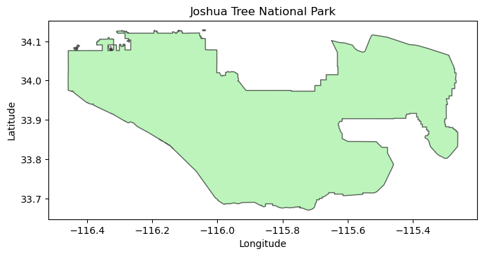
Step 4: Fetch Data with Coiled
Okay the real stuff. Here’s the flow:
Start cluster → spins up workers in us-west-1 (same region as the data)
Call
get_climate_data()→ workers fetch from S3, clip to your boundary, compute spatial averagesGet back DataFrames → results come back to your laptop as pandas DataFrames (in memory, not saved to disk)
Shut down cluster → important so you don’t burn credits
For 3 variables × 70 simulations × 5 years: ~1.5 min with Coiled vs ~30 min locally.
import coiled
import time
print("Starting cluster...")
t0 = time.perf_counter()

cluster = coiled.Cluster(
    name="tutorial-fetch",
    region="us-west1",                 # GCP region closest to S3 data in us-west-2
    n_workers=8,                       # 3 workers = fetch 3 vars in parallel
    worker_memory="16 GiB",             # each worker gets 8 GiB RAM
    spot_policy="spot_with_fallback",  # use spot instances (cheaper), fall back to on-demand if unavailable
    idle_timeout="5 minutes",          # shut down if idle (don't waste credits)
    package_sync=True,                 # sync local packages to workers (builds env automatically)
)

# this connects local python session to the remote scheduler
# all dask operations now run on the cluster, not laptop!
client = cluster.get_client()
print(f"\n✓ Ready in {time.perf_counter() - t0:.0f}s")
print(f"  Dashboard: {client.dashboard_link}")
Starting cluster...
/tmp/ipykernel_1033/735352309.py:6: FutureWarning: `package_sync` is a deprecated kwarg for `Cluster` and will be removed in a future release. To only sync certain packages, use `package_sync_only`, and to disable package sync, pass the `container` or `software` kwargs instead.
  cluster = coiled.Cluster(
✓ Ready in 218s
  Dashboard: https://cluster-pleiw.dask.host/LDM5fvRSJsHlQ2K4/status
# Fetch climate data using my library wrapper around calAdapt
# this gives work to the remote workers, they do the heavy lifting
print("Fetching data...")
t0 = time.perf_counter()

data = get_climate_data(
    variables=["T_Max", "T_Min", "Precip"],  # human-readable names (mapped to tasmax, tasmin, pr)
    scenarios=["Historical Climate"],         # mapped to "historical" experiment_id, all four would be: scenarios=["Historical Climate", "SSP 2-4.5", "SSP 3-7.0", "SSP 5-8.5"]
    boundary=boundary,                        # GeoDataFrame gets serialized to WKT automatically
    time_slice=(2010, 2014),                  # 5 years for demo-- keep it small to save credits
    timescale="monthly",                      # "monthly", "daily", or "yearly" (monthly is default)
    backend="coiled",                         # use Coiled cluster (vs "direct_s3" for local)
    coiled_cluster=cluster,                   # pass the cluster we just created
)

# data is a dict: {variable: DataFrame} where each DataFrame has all scenarios
print(f"\n✓ Done in {time.perf_counter() - t0:.1f}s")
print(f"  Got {len(data)} variables")
Fetching data...
✓ Done in 36.0s
Got 3 variables
# What did we get back? Let's peek at the structure

print("=== What `data` looks like ===")
print(f"Type: {type(data)}")
print(f"Keys: {list(data.keys())}")
print()

# Each key is a variable name, each value is a DataFrame with ALL scenarios
for var, df in data.items():
    print(f'data["{var}"] → DataFrame')
    print(f"    Shape: {df.shape[0]} rows × {df.shape[1]} cols")
    print(f"    Columns: {list(df.columns)}")
    print(f"    Scenarios in df: {df['scenario'].unique().tolist()}")
    print()
=== What `data` looks like ===
Type: <class 'dict'>
Keys: ['T_Max', 'T_Min', 'Precip']
data["T_Max"] → DataFrame
Shape: 4200 rows × 6 cols
Columns: ['simulation', 'time', 'spatial_ref', 'T_Max', 'scenario', 'timescale']
Scenarios in df: ['Historical Climate']
data["T_Min"] → DataFrame
Shape: 4200 rows × 6 cols
Columns: ['simulation', 'time', 'spatial_ref', 'T_Min', 'scenario', 'timescale']
Scenarios in df: ['Historical Climate']
data["Precip"] → DataFrame
Shape: 4200 rows × 6 cols
Columns: ['simulation', 'time', 'spatial_ref', 'Precip', 'scenario', 'timescale']
Scenarios in df: ['Historical Climate']
# Let's look inside one of those DataFrames
sample_df = data["T_Max"]

print("=== Inside the T_Max DataFrame ===")
print(f"Rows: {len(sample_df):,} (= 70 simulations × 60 months)")
print(f"Columns: {list(sample_df.columns)}")
print()
print("First 10 rows:")
sample_df.head(10)
=== Inside the T_Max DataFrame ===
Rows: 4,200 (= 70 simulations × 60 months)
Columns: ['simulation', 'time', 'spatial_ref', 'T_Max', 'scenario', 'timescale']

First 10 rows:
So each row is one month for one simulation. The T_Max column is the spatially-averaged max temperature (in °C) over Joshua Tree for that month.
Why 4,200 rows? → 70 simulations × 12 months × 5 years = 4,200
This is what we’ll save to CSV or plot directly.
# Always shut down the cluster!!!!
cluster.close()
print("Cluster shut down.")
Cluster shut down.
Part 2 recap
What just happened:
Started a cluster (3 workers on GCP us-west1)
Called
get_climate_data()which dispatched work to those workersWorkers fetched 70 Zarr stores from S3, clipped to Joshua Tree boundary, averaged spatially
Got back a
dictwith 3 DataFrames (one per variable), 12,600 total rowsAll in ~30 seconds
The data variable is now sitting in memory— we haven’t saved anything to disk yet. That comes later in Part 5.
Part 3: Key Library Functions
So now we’ll look at the key methods from my library built on top of climatekitae’s. Also, note that all the methods I’ve written are in lib/. This isn’t necessary for understanding how to get the data, it just is peeking under the hood.
get_climate_data() — The Main Function
This is prob what you’ll use most. It handles:
Mapping human-readable names → internal variable/experiment IDs
Serializing your shapefile boundary for remote workers
Dispatching fetches in parallel across the cluster
Clipping data to your boundary and averaging
Returning clean DataFrames
data = get_climate_data(
    variables=["T_Max", "T_Min", "Precip"],   # what to fetch
    scenarios=["Historical Climate"],          # which experiment(s)
    boundary=my_gdf,                           # GeoDataFrame of your area
    time_slice=(2010, 2020),                   # year range
    timescale="monthly",                       # "monthly", "daily", or "yearly"
    backend="coiled",                          # or "direct_s3" for locl
    coiled_cluster=cluster,                    # if using coiled
)
# returns: {"T_Max": DataFrame, "T_Min": DataFrame, "Precip": DataFrame}
What You Get Back
A dict mapping variable name → DataFrame. Each DataFrame has all the scenarios one reqeusted. Its a dict since its sort of standard at leastin my head to ask for t_max and t_min at the same time, and since there’s overhead to booting up a cluster, you can query multiple vars at once and seperate out the data in memory later-- though if you only ask for one variable, then you just get it through a dict with one entry. If I call data.get(“T_max”), I end up w/ a df that looks like:
| Column | Example | Description |
|---|---|---|
time | 2010-01-01 | Month of observation |
simulation | LOCA2_ACCESS-CM2_r1i1p1f1 | Climate model + run ID |
scenario | Historical Climate | Which experiment (historical, SSP, etc.) |
timescale | monthly | Temporal resolution of the data (sort of bloaty, but helps for no confusion) |
T_Max | 18.5 | The actual value (spatially averaged over your boundary) |
Scenario Options
| Friendly Name | Description |
|---|---|
"Historical Climate" | Past observations (1950-2014) |
"SSP 2-4.5" | Middle of the road (~2.7°C warming by 2100) |
"SSP 3-7.0" | Regional rivalry (~3.6°C warming by 2100) |
"SSP 5-8.5" | Fossil-fueled development (~4.4°C warming by 2100) |
Timescale Options
| timescale | Description | Variables | Data Size |
|---|---|---|---|
"monthly" | Monthly aggregates (default) | All 10 | Small |
"daily" | Daily values | All 10 | ~30x larger |
"yearly" | Annual maximum only | T_Max only | Tiny |
How Aggregation Works (from Cal-Adapt/LOCA2)
Cal-Adapt’s LOCA2 data is natively daily. Monthly values are pre-aggregated:
| Variable | Monthly Aggregation | Units |
|---|---|---|
| Temperature (T_Max, T_Min) | Mean of daily values | °C |
| Precipitation | Sum of daily values | mm/month |
| Humidity, Wind, Radiation | Mean of daily values | various |
Yearly (yrmax) is special — it’s the hottest day of the year (max of daily T_Max), not an annual mean. Only T_Max is available at this timescale.
Note: If you request a variable that doesn’t exist at the chosen timescale (e.g., Precip at yearly), you’ll get a helpful error message telling you what’s available.
Live Example: Fetching One Variable
Let’s see this in action. We’ll fetch just T_Max for a short time range and look at the DataFrame we get back.
Note: This uses the data we already fetched in Part 2, so no new cluster needed!
# Using the data we fetched in Part 2, let's look at T_Max
# (If you skipped Part 2, you'll need to run those cells first)

# The dict key is just the variable name now!
tmax_df = data["T_Max"]

print("=== DataFrame from get_climate_data() ===")
print(f"Type: {type(tmax_df)}")
print(f"Shape: {tmax_df.shape[0]} rows × {tmax_df.shape[1]} columns")
print(f"Columns: {list(tmax_df.columns)}")
print()
print("First 10 rows:")
tmax_df.head(10)
=== DataFrame from get_climate_data() ===
Type: <class 'pandas.DataFrame'>
Shape: 4200 rows × 6 columns
Columns: ['simulation', 'time', 'spatial_ref', 'T_Max', 'scenario', 'timescale']
First 10 rows:
# Each row = one month × one simulation
# print to see what's in each column

print("=== Column breakdown ===")
print(f"time: {tmax_df['time'].dtype}")
print(f"  Range: {tmax_df['time'].min()} to {tmax_df['time'].max()}")
print()
print(f"simulation: {tmax_df['simulation'].dtype}")
print(f"  Unique values: {tmax_df['simulation'].nunique()}")
print(f"  Examples: {tmax_df['simulation'].unique()[:3].tolist()}")
print()
print(f"scenario: {tmax_df['scenario'].dtype}")
print(f"  Unique values: {tmax_df['scenario'].unique().tolist()}")
print()
print(f"T_Max: {tmax_df['T_Max'].dtype}")
print(f"  Range: {tmax_df['T_Max'].min():.1f}°C to {tmax_df['T_Max'].max():.1f}°C")
print(f"  Mean: {tmax_df['T_Max'].mean():.1f}°C")
=== Column breakdown ===
time: datetime64[ns]
Range: 2010-01-01 00:00:00 to 2014-12-01 00:00:00
simulation: str
Unique values: 70
Examples: ['LOCA2_ACCESS-CM2_r1i1p1f1', 'LOCA2_ACCESS-CM2_r2i1p1f1', 'LOCA2_ACCESS-CM2_r3i1p1f1']
scenario: str
Unique values: ['Historical Climate']
T_Max: float32
Range: 9.5°C to 40.9°C
Mean: 26.5°C
So that’s what you get back from get_climate_data() — a clean pandas DataFrame with 4 columns that’s ready for analysis or export to CSV.
CatalogExplorer.s3_paths() — Where the Data Lives
Each variable/scenario combo has ~70 Zarr stores on S3, one per climate model simulation.
# s3_paths returns the actual S3 bucket locations
paths = cat.s3_paths("tasmax", "historical")
print(f"{len(paths)} Zarr stores for tasmax/historical")
print()
print("First 3:")
for p in paths[:3]:
    print(f"  {p['source_id']:15s} → {p['path']}")
70 Zarr stores for tasmax/historical
First 3:
ACCESS-CM2 → s3://cadcat/loca2/ucsd/access-cm2/historical/r1i1p1f1/mon/tasmax/d03/
ACCESS-CM2 → s3://cadcat/loca2/ucsd/access-cm2/historical/r2i1p1f1/mon/tasmax/d03/
ACCESS-CM2 → s3://cadcat/loca2/ucsd/access-cm2/historical/r3i1p1f1/mon/tasmax/d03/
boundary_to_wkt() — Seralises Geometry
Problem: We send tasks to remote workers (the guys that live on coiled + AWS). It’s sort of interesting, but you have to seralise your functions which are then decoded on the coiled workers-- this is of course, since they’re not using MacOS, and this provides platform indpendence. For most things, you can just put imports and normal python code and let pickle 🥒 (a library) send it through to remote workers. However, GeoDataFrames contain C objects that can’t be serialized (huge painful bug).
Solution: Convert to WKT (Well-Known Text) strings, reconstruct on the worker (pretty stoked on this work around 🌊).
from andrewAdaptLibrary import boundary_to_wkt, boundary_from_wkt

# Convert to strings (this is what we send to remote workers)
wkt_list, crs_str = boundary_to_wkt(boundary)
print(f"CRS: {crs_str}")
print(f"WKT (first 150 chars): {wkt_list[0][:150]}...")

# Reconstruct on the other side (this happens on the remote worker)
reconstructed = boundary_from_wkt(wkt_list, crs_str)

# verify it worked - compare geometry bounds instead of area (area calc warns about geographic CRS)
orig_bounds = boundary.total_bounds
recon_bounds = reconstructed.total_bounds
print(f"\nRound-trip OK: {all(abs(o - r) < 1e-6 for o, r in zip(orig_bounds, recon_bounds))}")
CRS: EPSG:4326
WKT (first 150 chars): MULTIPOLYGON (((-116.326942 34.078087, -116.326933 34.079128, -116.326933 34.079895, -116.325847 34.079895, -116.325855 34.078079, -116.326942 34.0780...
Round-trip OK: True
fetch_direct_s3() — Lazy Arrays
This opens Zarr stores but doesn’t download data yet. Data only moves when you call .load().
from andrewAdaptLibrary import fetch_direct_s3

# Open Zarr stores (lazy — no download yet)
lazy = fetch_direct_s3(
    var_key="T_Max",
    experiment="historical",
    time_slice=(2010, 2010),  # Just 1 year
    lat_bounds=lat_bounds,
    lon_bounds=lon_bounds,
    catalog=cat,
)

print(f"Shape: {lazy.shape}")
print(f"Dims: {lazy.dims}")
print(f"Size if loaded: {lazy.nbytes / 1e6:.1f} MB")
print()
print("No data downloaded yet! Call .load() to fetch.")
Shape: (70, 12, 15, 39)
Dims: ('simulation', 'time', 'lat', 'lon')
Size if loaded: 2.0 MB
No data downloaded yet! Call .load() to fetch.
Part 3 done.
Key concepts:
Live catalog —
CatalogExplorerqueries real data, not hardcoded listsWKT serialization — geometry converted to strings for remote workers
Lazy arrays — Zarr stores opened without downloading; data fetched on
.load()
Part 4: More walkthroughs & now exersises!
# Example: looking up a park and running the full pipeline

def analyze_park(park_name, variables, scenarios, years, timescale="monthly", n_workers=3):
    """
    Template function for analyzing any park/region.

    Args:
        park_name: exact NPS unit name (use catalog.search() to find it)
        variables: list of ["T_Max", "T_Min", "Precip"]
        scenarios: list of ["Historical Climate", "SSP 2-4.5", "SSP 3-7.0", "SSP 5-8.5"]
        years: tuple like (2010, 2020)
        timescale: "monthly", "daily", or "yearly" (default "monthly")
        n_workers: how many parallel workers (default 3)
    """
    import coiled

    # 1. Load the boundary from the mega NPS shapefile
    boundary = catalog.get_boundary(park_name)
    print(f"Loaded boundary for {park_name}: {len(boundary)} polygon(s)")

    # check it's in CA roughly
    lat_bounds, lon_bounds = get_lat_lon_bounds(boundary)
    if lat_bounds[0] < 32 or lat_bounds[1] > 42:
        print("Warning: latitude outside CA range (32-42°N)")
    if lon_bounds[0] < -125 or lon_bounds[1] > -114:
        print("Warning: longitude outside CA range (125-114°W)")

    # 2. Start cluster
    cluster = coiled.Cluster(
        name="custom-park-analysis",
        region="us-west1",
        n_workers=n_workers,
        worker_memory="8 GiB",
        spot_policy="spot_with_fallback",
        idle_timeout="10 minutes",
        package_sync=True,             # sync local packages to workers
    )
    client = cluster.get_client()

    try:
        # 3. Fetch data
        data = get_climate_data(
            variables=variables,
            scenarios=scenarios,
            boundary=boundary,
            time_slice=years,
            timescale=timescale,
            backend="coiled",
            coiled_cluster=cluster,
        )
        return data
    finally:
        # 4. Always shut down
        cluster.close()
        print("Cluster shut down.")

#  (don't run this— just an example):
# data = analyze_park(
#     park_name="Death Valley National Park",
#     variables=["T_Max", "T_Min"],
#     scenarios=["Historical Climate", "SSP 5-8.5"],
#     years=(2015, 2025),
#     timescale="monthly",  # or "daily" for extreme event analysis
# )
Exercise 1: Start a Coiled Cluster
Fill in the blanks to create a cluster on GCP in the region closest to the Cal-Adapt data.
Note: We use package_sync=True which automatically syncs your local Python packages to the workers — no need to specify a software environment!
import coiled

# Fill in the blanks
cluster = coiled.Cluster(
    name="exercise-cluster",
    region="____",             # hint: GCP region closest to the S3 data
    n_workers=2,
    worker_memory="8 GiB",     # this is filled in since coiled gets mad if you choose non-standard sizes
    idle_timeout="____ minutes",  # hint: don't waste credits
    package_sync=True,         # this syncs your local packages to workers
)
client = cluster.get_client()
print(f"Dashboard: {client.dashboard_link}")
# Check: if the cluster started, you're good!
print(f"Workers: {len(client.scheduler_info()['workers'])}")
print("Exercise 1 done!")# SOLUTION
import coiled
cluster = coiled.Cluster(
name="exercise-cluster",
region="us-west1", # GCP region closest to S3 data
n_workers=2,
worker_memory="8 GiB",
idle_timeout="5 minutes", # any reasonable timeout works
package_sync=True, # sync local packages to workers
)
client = cluster.get_client()
print(f"Dashboard: {client.dashboard_link}")Exercise 2: Fetch Climate Data
Use get_climate_data() to fetch T_Max for Joshua Tree from 2015-2019:
# Load boundary from the mega NPS shapefile
jt_boundary = catalog.get_boundary("Joshua Tree National Park")

# Fill in the blanks
data = get_climate_data(
    variables=["____"],              # hint: max temperature
    scenarios=["____"],              # hint: past observations
    boundary=____,                   # hint: variable we just loaded
    time_slice=(2015, ____),         # hint: 5 years ending in 2019
    backend="____",                  # hint: use the cloud
    coiled_cluster=____,             # hint: the cluster we started above
)
# Check your answer
def check_ex2(data):
assert "T_Max" in data, f"Expected 'T_Max' key, got {list(data.keys())}"
df = data["T_Max"]
assert len(df) > 0, "DataFrame is empty"
years = df['time'].dt.year.unique()
assert 2015 in years and 2019 in years, f"Wrong years: {years}"
print(f"Exercise 2 done. {len(df)} rows fetched.")
check_ex2(data)# SOLUTION
jt_boundary = catalog.get_boundary("Joshua Tree National Park")
data = get_climate_data(
variables=["T_Max"],
scenarios=["Historical Climate"],
boundary=jt_boundary,
time_slice=(2015, 2019),
timescale="monthly",
backend="coiled",
coiled_cluster=cluster,
)
print(f"Got {len(data)} result(s)")Part 5: Working with the Data, using R as well
Now that data has been fetched, here’s how to explore it and save it for analysis in R or elsewhere.
What’s in the DataFrame?
get_climate_data() returns a dict of DataFrames. Let’s peek at what we actually get back:
# grab one of the dataframes we fetched earlier
# data is a dict like: {"T_Max": DataFrame, "T_Min": DataFrame, ...}
sample_df = data["T_Max"]

print("=== DataFrame Structure ===")
print(f"Shape: {sample_df.shape[0]} rows × {sample_df.shape[1]} columns")
print(f"\nColumns: {list(sample_df.columns)}")
print(f"\nData types:")
print(sample_df.dtypes)
print(f"\n=== First 5 rows ===")
sample_df.head()
Column Meanings
So note right now this is like saving data for if we’re going to do a timeseries like temperature over the park, not 3km specific boxes-- still trying to set up the most elegant methods and such for spatial plotting on the parks.
| Column | Type | Description |
|---|---|---|
time | datetime | Month of observation (e.g., 2010-01-01 = January 2010) |
simulation | string | Climate model + run ID (e.g., “LOCA2_ACCESS-CM2_r1i1p1f1”) |
scenario | string | The climate scenario (e.g., “Historical Climate”, “SSP 3-7.0”) |
timescale | string | Temporal resolution: “monthly”, “daily”, or “yearly” |
T_Max / T_Min / Precip | float | The actual climate value, spatially averaged over your boundary |
Each row = one month × one simulation. So 5 years × 12 months × 70 simulations = 4,200 rows.
Why include scenario and timescale in the DataFrame? So the DataFrame is fully self-describing. If you load a CSV 6 months later, you’ll know exactly what data it contains without checking filenames.
# quick stats
print("=== Quick Stats ===")
print(f"Time range: {sample_df['time'].min()} to {sample_df['time'].max()}")
print(f"Unique simulations: {sample_df['simulation'].nunique()}")
print(f"\nT_Max summary (°C):")
print(sample_df['T_Max'].describe())
Saving to CSV (for R)
Remember that this project is set up such that we have an R kernel w/ Juptyr notebooks ready to go, you can make a notebook and then use and R kernel to plot the data we’re saving to csv.
The DataFrames are standard pandas— save them however you want:
# Option 1: Save each variable separately
import os
output_dir = os.path.join(PROJECT_ROOT, "data", "processed")
os.makedirs(output_dir, exist_ok=True)

for var, df in data.items():
    # clean filename: "T_Max.csv"
    filename = f"{var}.csv"
    filepath = os.path.join(output_dir, filename)
    df.to_csv(filepath, index=False)
    print(f"Saved: {filename} ({len(df)} rows)")

print(f"\nFiles saved to: {output_dir}")
# Option 2: Combine all variables into one tidy dataframe
import pandas as pd
# Each DataFrame already has 'scenario' column, just add 'variable' and rename value col
tidy_dfs = []
for var, df in data.items():
df_copy = df.copy()
df_copy['variable'] = var
df_copy = df_copy.rename(columns={var: 'value'}) # generic 'value' column
tidy_dfs.append(df_copy)
tidy_df = pd.concat(tidy_dfs, ignore_index=True)
print(f"Combined shape: {tidy_df.shape}")
print(f"Columns: {list(tidy_df.columns)}")
tidy_df.head()# save the tidy version
tidy_path = os.path.join(output_dir, "climate_data_tidy.csv")
tidy_df.to_csv(tidy_path, index=False)
print(f"Saved: {tidy_path}")Reading in R
Super simple once we have the csv’s, with the file struct that we have in the notebook an exmaple notebook would look like this:
library(tidyverse)

# read one file
tmax <- read_csv("data/processed/T_Max_Historical_Climate.csv")

# or the tidy combined version
climate <- read_csv("data/processed/climate_data_tidy.csv")

# quick plot
climate %>%
  filter(variable == "T_Max") %>%
  group_by(time) %>%
  summarise(mean_temp = mean(value), .groups = "drop") %>%
  ggplot(aes(x = time, y = mean_temp)) +
  geom_line() +
  labs(title = "Mean Max Temp across simulations", y = "°C")
TL;DR — Copy-Paste Minimal Example
Overview each step:
| Step | What you do | What you get back |
|---|---|---|
ParkCatalog(shp) | Load the mega NPS shapefile | ParkCatalog with ~437 NPS units |
catalog.get_boundary(name) | Get a park boundary | GeoDataFrame with your park boundary |
coiled.Cluster(...) | Spin up cloud workers | Cluster object (workers running in Oregon) |
get_climate_data(...) | Fetch + clip + average | dict of {variable: DataFrame} |
cluster.close() | Shut down workers | Nothing |
Each DataFrame has columns: simulation, time, spatial_ref, <variable>, scenario, timescale
# === Minimal ex: Fetch 5 years of climate data for any park ===
import os, coiled
from andrewAdaptLibrary import ParkCatalog, get_climate_data

PROJECT_ROOT = os.path.abspath(os.path.join(os.getcwd(), "..", ".."))
NPS_SHP = os.path.join(
    PROJECT_ROOT,
    "USA_National_Park_Service_Lands_20170930_4993375350946852027",
    "USA_Federal_Lands.shp",
)

# 1. Look up your park in the mega NPS shapefile → returns GeoDataFrame
catalog = ParkCatalog(NPS_SHP)
boundary = catalog.get_boundary("Joshua Tree National Park")

# 2. Spin up cluster → returns Cluster object (workers now running in GCP us-west1)
cluster = coiled.Cluster(
    name="quick-fetch",
    region="us-west1",
    n_workers=3,
    worker_memory="8 GiB",
    spot_policy="spot_with_fallback",
    idle_timeout="10 minutes",
    package_sync=True,
)

# 3. Fetch data → returns {variable_name: DataFrame}
data = get_climate_data(
    variables=["T_Max"],
    scenarios=["Historical Climate"],
    boundary=boundary,
    time_slice=(2010, 2014),
    timescale="monthly",
    backend="coiled",
    coiled_cluster=cluster,
)

# 4. Shut down cluster
cluster.close()

# 5. Use the data
df = data["T_Max"]
print(df.head())
What you end up with
After running the above, data is a Python dict sitting in memory:
data = {
    "T_Max": DataFrame with columns [time, simulation, scenario, timescale, T_Max],
    "T_Min": DataFrame with columns [time, simulation, scenario, timescale, T_Min],
    "Precip": DataFrame with columns [time, simulation, scenario, timescale, Precip],
}
Each DataFrame has:
All scenarios combined — if you requested Historical + SSP 3-7.0, both are in the same DataFrame
~4,200 rows per scenario (5 years × 12 months × 70 simulations)
5 columns:
time,simulation,scenario,timescale, and the variable value
To get just one scenario:
tmax_df = data["T_Max"]
historical_only = tmax_df[tmax_df["scenario"] == "Historical Climate"]
From here you can:
Plot directly in Python with matplotlib/seaborn
Save to CSV with
df.to_csv("myfile.csv")Analyze with pandas (groupby, resample, etc)
Pass to R by saving CSV then
read_csv()in R